Surrogates & Bayesian optimization (Layer 5)

When each evaluation is expensive (a GetDP solve, a transient FEA run, a dyno test), the roughly 10³ evaluations a genetic algorithm needs are not affordable. Bayesian optimization finds comparable designs in tens of evaluations by spending compute on deciding where to evaluate next.

Code: axfluxmdo.optimize.dataset, surrogate, bayesopt, axfluxmdo.viz.bayesopt. Requires pip install "axfluxmdo[opt]" (scikit-learn + scipy).

---

1. Gaussian-process regression in five lines

Given \(n\) observations \(\mathbf y\) at inputs \(X\), a GP with kernel \(k(\cdot,\cdot)\) predicts at a new point \(x_*\):

\[ \mu(x_*) = \mathbf k_*^\top (K + \sigma_n^2 I)^{-1}\, \mathbf y , \qquad \sigma^2(x_*) = k(x_*,x_*) - \mathbf k_*^\top (K + \sigma_n^2 I)^{-1} \mathbf k_* , \]

where \(K_{ij} = k(x_i, x_j)\) and \((\mathbf k_*)_i = k(x_i, x_*)\). The mean interpolates the data, and the variance grows away from it. That variance is the quantity that drives exploration.

The kernel is a Matérn-5/2 with ARD (automatic relevance determination, meaning one length scale per input dimension):

\[ k(x, x') = \sigma_f^2 \Big(1 + \sqrt5 d + \tfrac53 d^2\Big) e^{-\sqrt5 d}, \qquad d^2 = \sum_j \frac{(x_j - x_j')^2}{\ell_j^2} . \]

ARD matters here because the feature encoding mixes scales (meters, unitless fill factors, ordinal pole counts), and per-dimension \(\ell_j\) let the GP learn each variable's influence after standardization. Length scales are fit by maximizing the marginal likelihood; trustworthiness is judged by k-fold cross-validation (cv_rmse/cv_r2), not by the optimizer's convergence warnings.

2. Expected improvement, derived

Let \(y^\*\) be the best (minimize-space) value observed so far. The improvement at \(x\) is \(\max(0,\ y^\* - Y)\) where \(Y \sim \mathcal N(\mu, \sigma^2)\) is the GP's belief. Its expectation:

\[ \mathrm{EI}(x) = \mathbb E\big[\max(0, y^* - Y)\big] = \int_{-\infty}^{y^*} (y^* - y)\, \phi\!\Big(\frac{y-\mu}{\sigma}\Big)\frac{dy}{\sigma} . \]

Substituting \(z = (y^\* - \mu - \xi)/\sigma\) (with a small exploration margin \(\xi\)) and integrating by parts:

\[ \boxed{\; \mathrm{EI}(x) = (y^* - \mu - \xi)\,\Phi(z) \;+\; \sigma\,\phi(z) \;} \]

The two terms have direct interpretations: exploitation (probability-weighted improvement of the mean) plus exploration (reward for uncertainty). EI goes to zero as \(\sigma \to 0\), so the optimizer does not re-evaluate points it already knows. The acquisition is maximized over a seeded candidate pool (half uniform, half perturbations of the incumbent), which is derivative-free and correct for the mixed continuous/integer/choice space.

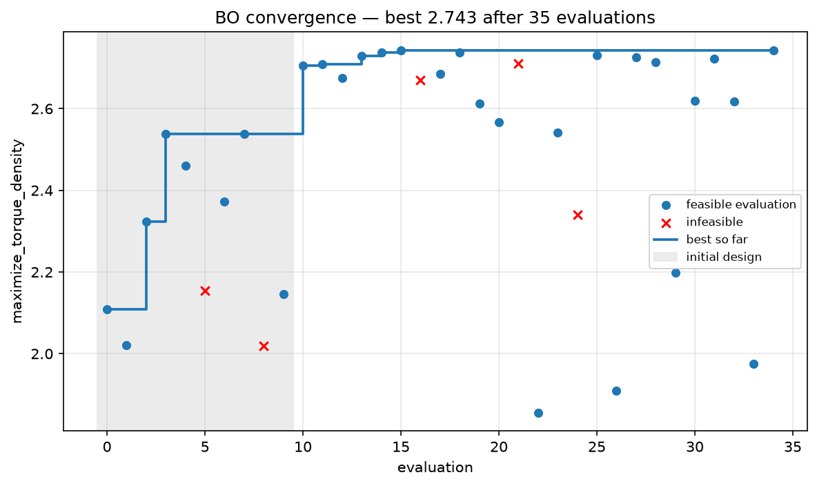
3. The loop

1. Initial design: a Latin hypercube over the continuous/integer box. Stratified sampling guarantees one-dimensional coverage that i.i.d. uniform sampling does not. Choice variables use seeded random draws.
2. Fit the GP. Infeasible points receive a soft penalty (worst feasible value plus 10% of the feasible range) rather than the 10⁹ geometry penalty, which would destroy the smoothness the GP depends on.
3. Maximize EI, evaluate the winner, and append it to the DesignDataset (JSON Lines with a versioned header, so every evaluation is a permanent artifact).
4. Repeat. The same seed produces an identical trajectory (test-pinned).

On the reference problem, BO reaches the genetic algorithm's torque-density optimum in 35 evaluations versus roughly 1200, and slightly exceeds it because the local perturbation pool polishes the incumbent.

4. Uncertainty-aware recommendation

BOStudy.recommend(k, risk_aversion=κ) ranks evaluated, verified-feasible designs by the pessimistic score \(\mu - \kappa\sigma\) (maximize sense). A design the surrogate is unsure about ranks below a slightly worse one with verified neighbors. The ranking covers only evaluated designs; it makes no claim about unevaluated space.

5. Expensive objectives

Any callable can be the objective; the cheap model still supplies the constraints:

from axfluxmdo.solvers import solve_open_circuit

def fea_b1(motor, op):
    return {"fea_b1_t": solve_open_circuit(motor, magnet_temp_c=65.0).fundamental_b1_t}

study = bayesian_optimize(
    motor, op,
    variables={"magnet_thickness": (0.002, 0.008), "air_gap": (0.0005, 0.0015)},
    objective="maximize_fea_b1_t",
    expensive_fn=fea_b1,
    n_initial=6, n_iterations=12,
)

---

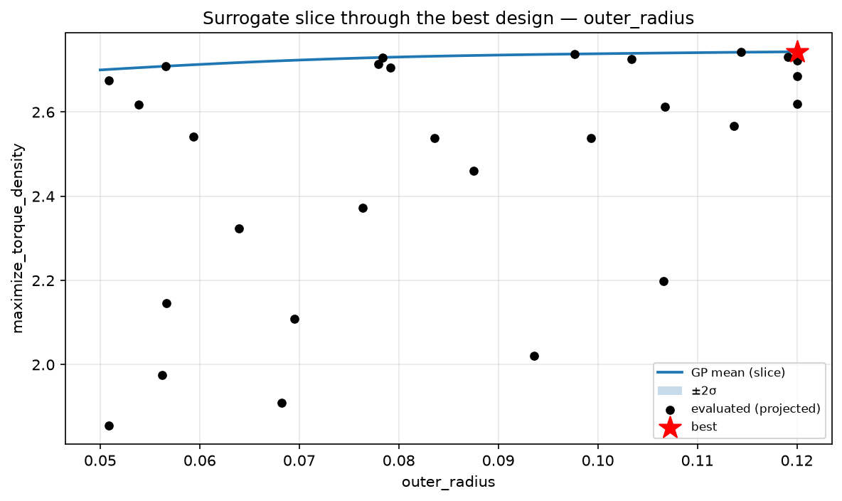
See example 07 for the 35-evaluation study, convergence and surrogate-slice plots, the dataset round-trip, and the FEA-objective recipe.