The 2.5D annular model (Layer 2)

The annular model splits the disk machine into radial slices and evaluates the field, torque contribution, yoke loading, and core loss per slice. It adds the physics that is genuinely radius-dependent and nothing else, which is why it agrees with the analytical model to machine precision for a perfect machine.

Code: axfluxmdo.models.annular_2p5d, axfluxmdo.geometry.tolerances, axfluxmdo.materials.magnetic (runout averages).

---

1. Why the slice sum is exact, not approximate

For slice \(k\) with exact annulus area \(dA_k = \pi(r_{k+1}^2 - r_k^2)\), the per-slice flux linkage is

\[ d\lambda_k = \frac{k_w N\, B_1(r_k)\, dA_k}{\pi p}, \qquad \lambda = \sum_k d\lambda_k . \]

Torque and EMF come from the summed \(\lambda\) exactly as in Layer 1. Because the analytical model's \(\lambda \propto B_1 A_g\) is linear in area, and \(\sum_k dA_k = A_g\) exactly, a radius-uniform \(B_1\) gives the identical \(\lambda\) at any slice count, with no discretization error at all. Only quantities nonlinear in radius (core loss via \(B_y(r)^{1.68}\), the saturation maximum) are discretized, and they converge fast. The test suite pins single-slice parity on every output key at 10⁻¹² relative.

The energy identity \(m E I = T \omega_m\) survives unchanged because both quantities still derive from the one summed \(\lambda\), per slice and in aggregate.

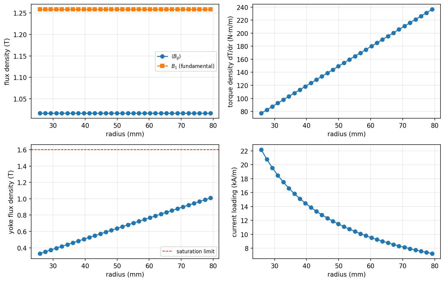
2. Radius-dependent yoke loading: why saturation binds at \(r_o\)

The local pole pitch grows with radius, \(\tau_p(r) = \pi r / p\), so each pole's flux return through the yoke grows too:

\[ B_y(r) \;=\; \frac{B_g(r)\,\alpha(r)\, \pi r}{2\, p\, t_\mathrm{core}\, k_\mathrm{stack}} . \]

The yoke flux density is largest at the outer radius, so the analytical model's mean-radius proxy underestimates the true maximum. The annular model's saturation constraint uses \(\max_k B_y(r_k)\); the practical consequence appeared immediately in validation: a \(p = 8\) variant that Layer 1 called feasible saturates at 1.77 T at \(r_o\) against a 1.6 T limit.

3. Manufacturing imperfections

GapImperfections models three deviations of the running gap (all in meters, attached to the motor so they sweep and optimize like any design variable):

\[ g(r, \theta) = g_0 + \underbrace{\Delta g}_{\text{offset}} + \underbrace{c\,\frac{r - r_m}{r_o - r_i}}_{\text{coning}} + \underbrace{\delta \cos\theta}_{\text{runout}} . \]

Offset and coning are axisymmetric, so they enter the per-slice load line directly. Runout varies around the circumference and needs an average.

The runout average, in closed form

The load line is a Möbius function of the gap, \(B(g) = B_r h_m / (a + b\cos\theta)\) with \(a = h_m + \mu_r \bar g\) and \(b = \mu_r \delta\). Its circumferential mean uses the classic integral

\[ \frac{1}{2\pi}\int_0^{2\pi} \frac{d\theta}{a + b\cos\theta} = \frac{1}{\sqrt{a^2 - b^2}} , \]

giving

\[ \langle B \rangle_\theta \;=\; \frac{B_r\, h_m}{\sqrt{(h_m + \mu_r \bar g)^2 - (\mu_r\delta)^2}} . \]

The counterintuitive sign: Jensen's inequality

\(B(g)\) is convex in \(g\) (second derivative positive). Jensen's inequality then guarantees

\[ \langle B(\bar g + \delta\cos\theta) \rangle \;\ge\; B(\bar g) : \]

runout slightly increases mean flux and mean torque. The closed form confirms it, since \(\sqrt{a^2-b^2} < a\). Runout's real penalties are elsewhere:

• a 1/rev torque modulation, reported as torque_ripple_proxy \(= (\lambda_+ - \lambda_-)/(\lambda_+ + \lambda_-)\) from the gap extremes;
• axial-force modulation on the bearings.

This sign is test-pinned. If a future change makes runout reduce mean torque, the model is wrong, not the test.

4. Axial force from the Maxwell stress tensor

The magnetic normal stress on the stator face is \(B^2/2\mu_0\). Integrated over the magnet-covered annulus:

\[ F_z \;=\; \sum_k \frac{\langle B_g^2\rangle_k}{2\mu_0}\, \alpha_k\, dA_k , \]

with \(\langle B^2\rangle\) also closed-form under runout (\(\propto a/(a^2-b^2)^{3/2}\)). For the reference motor this is about 5.6 kN of one-sided pull, the defining mechanical burden of a single-gap topology; a double-gap machine balances it. The result string reports this explicitly.

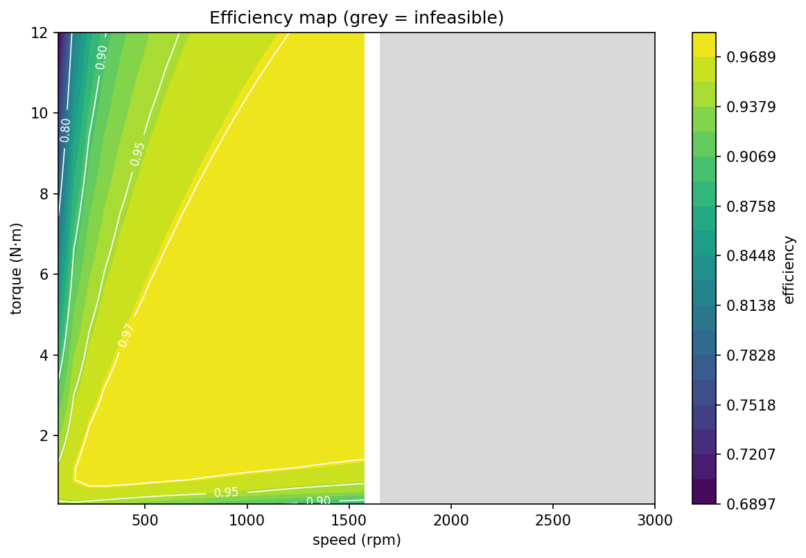
5. Efficiency maps

Because the model has no saturation, torque is linear in current and torque-per-amp is speed-independent: one probe evaluation inverts the map, then each (speed, torque) cell is a single model call. Cells violating any constraint are masked, with the first binding constraint recorded. The grey wall in the reference map near 1650 rpm is the 48 V bus voltage limit, at the speed the back-EMF predicts.

---

See example 03 for the parity demo, radial profiles, and efficiency map, and example 04 for gap error, coning, runout (including the Jensen sign), and magnet-arc sweeps.