axfluxmdo
Parametric modeling, simulation, visualization, and multidisciplinary design optimization of axial-flux permanent-magnet motors.

![]()
![]()
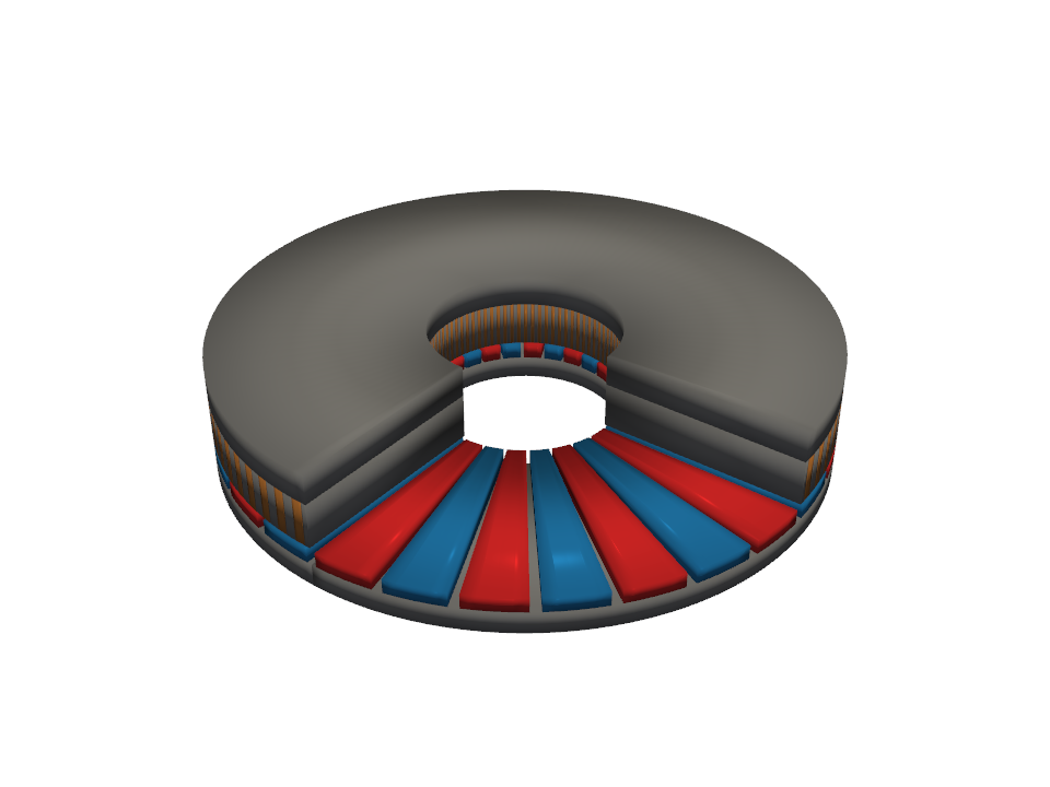
axfluxmdo is a design-exploration layer for axial-flux machines. It does not
replace expert designers or high-fidelity FEA; it supplies the fast, validated
models around them: parametric geometry, closed-form and 2.5D physics,
open-source solver automation, and Pareto-front and Bayesian optimization, so
that design tradeoffs are quantified early.
What's inside
| Layer | What it does | Evaluation cost |
|---|---|---|
| Analytical model | Closed-form torque, back-EMF, losses, thermal, constraints | microseconds |
| 2.5D annular model | Radius-resolved fields, manufacturing imperfections, ripple, axial force, efficiency maps | microseconds–ms |
| Pareto optimization | Mixed-variable NSGA-style fronts, sensitivities, OpenMDAO | seconds per study |
| FEA validation | Gmsh + GetDP open-circuit solves, sim-to-analytical residuals | seconds per solve |
| Surrogates + BO | GP surrogates, expected-improvement loops for expensive objectives | tens of evaluations |
| 3D visualization | PyVista assemblies and animations | — |
Every layer validates against the one below it: the annular model reproduces the analytical model to machine precision in its limit, and the analytical load line is checked against open-source FEA. The measured residuals are published in Limitations.

Example
from axfluxmdo import AxialFluxMotor, OperatingPoint
from axfluxmdo.models import AnalyticalModel

motor = AxialFluxMotor(
    outer_radius=0.08, inner_radius=0.025, air_gap=0.0008, pole_pairs=14,
)
op = OperatingPoint(speed_rpm=500, current_rms=25, dc_bus_voltage=48)
result = AnalyticalModel().evaluate(motor, op)
print(result)   # torque, efficiency, winding temp, constraint margins...
Continue with Getting Started, browse the worked examples, or jump to the API reference.