FEA validation (Layer 3 solvers)¶

The package never reimplements FEM. It generates geometry and meshes with Gmsh, drives GetDP (open-source magnetostatics) on them, and compares the result against its own analytical layer. The measured residuals are part of the documentation.

Code: axfluxmdo.solvers.gmsh_export, getdp_runner, results_parser, axfluxmdo.validation.sim2real. Requires pip install "axfluxmdo[fea]" + the GetDP binary.

1. The 2D unrolled approximation¶

Axial-flux machines are inherently 3D, but unrolling the annulus at the mean radius \(r_m\) turns one pole pair into a 2D planar problem: \(x\) is the circumferential coordinate over \(2\tau_p\), \(y\) is axial, and the model is periodic in \(x\). The approximation is good when the radial build \((r_o - r_i)\) is several times the pole pitch and field quantities vary slowly with radius. This is the same regime where the annular model treats radius as a parameter, not a field variable. Radial end effects are outside its scope.

2. The magnetostatic formulation¶

In 2D the flux density derives from a single vector-potential component \(A_z\): \(\mathbf B = \nabla \times (A_z \hat z)\), which satisfies \(\nabla\cdot\mathbf B = 0\) identically. With reluctivity \(\nu = 1/\mu\) and a permanent-magnet source of remanence \(\mathbf B_r\), Ampère's law becomes

\[ \nabla \times \big( \nu\, (\nabla \times A_z\hat z - \mathbf B_r) \big) = 0 , \]

whose weak (Galerkin) form is what the generated GetDP .pro file states: find \(A_z\) such that for all test functions \(w\),

\[ \int_\Omega \nu\, \nabla A_z \cdot \nabla w \; d\Omega \;=\; \int_{\Omega_m} \nu\, \mathbf B_r \cdot (\nabla \times w\hat z)\; d\Omega . \]

The magnet constitutive law in the template, \(\mathbf B = \mu_0\mu_r \mathbf H + \mathbf B_r\), is the identical recoil line behind the analytical load line. Any residual between FEA and the load line is therefore geometric (leakage, fringing, finite iron \(\mu\)) rather than a material-model discrepancy.

Boundary conditions: \(A_z = 0\) on the outer iron backs (flux confined), periodic linking of the left/right edges (which requires the mesh nodes to match; the exporter enforces matched periodic meshing, and a conformality test guards against cracked interfaces).

3. What the FEA measured¶

Gap field comparison

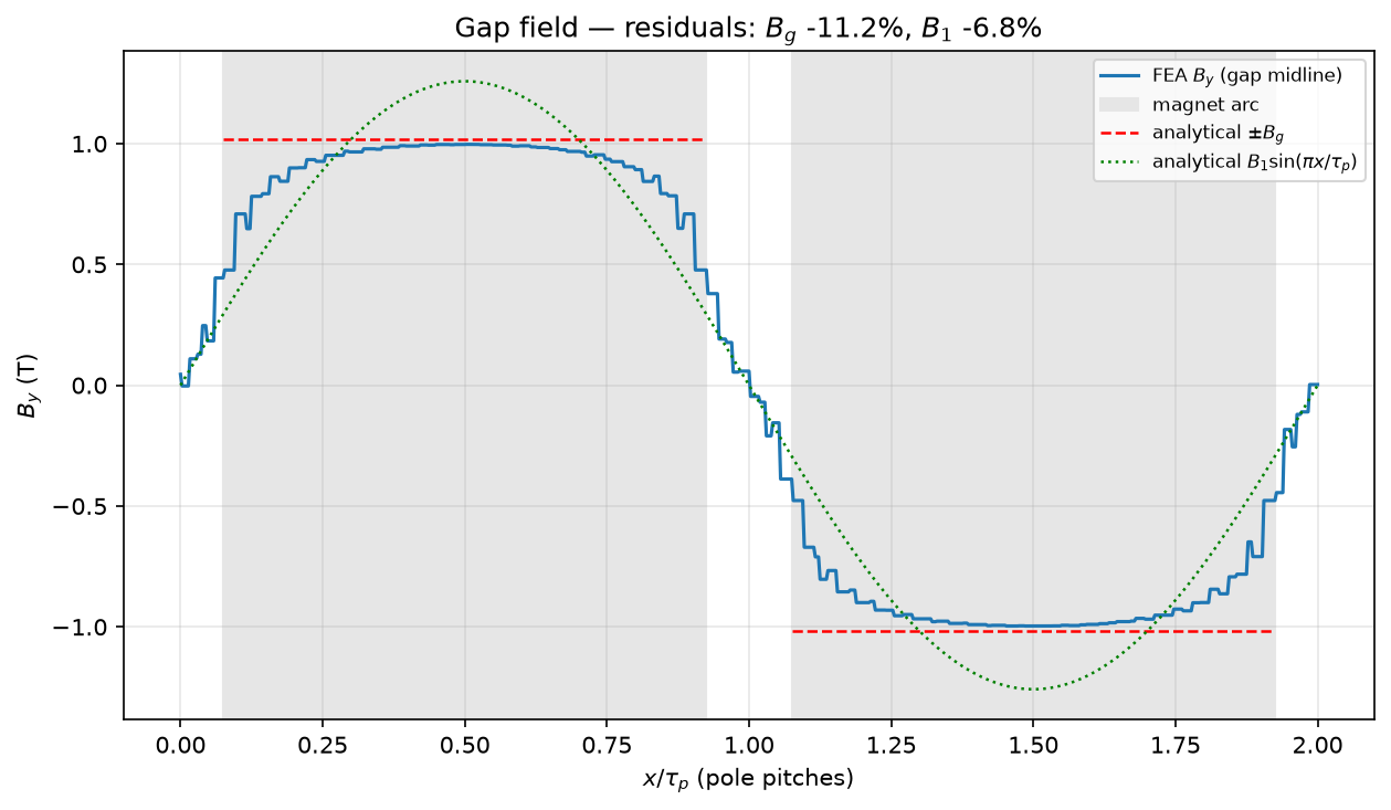
For the reference motor (slotless face, identical materials):

under-magnet mean: −11.2% vs the load line \(B_g\),
fundamental: −6.8% vs \(B_1\).

The flat top sits just below the analytical line. The shoulders, where flux spreads circumferentially as it crosses the gap and leaks pole-to-pole between magnets, are what the 1D circuit cannot represent. The load line is an upper bound, and the error bars are now measured.

4. Carter factor: theory vs measurement¶

Classical Carter theory corrects the effective gap for slot openings:

\[ k_C = \frac{\tau_s}{\tau_s - \gamma g}, \qquad \gamma = \frac{(w/g)^2}{5 + w/g}, \]

with slot pitch \(\tau_s\) and opening width \(w\). For this stator (\(w/g \approx 2.5\)) it predicts \(k_C \approx 1.2\). The measured value is \(k_C = 1.44\), because the classical formula assumes shallow, semi-closed slots while this machine has fully open slots as deep as the winding window.

The measurement itself cancels the fringing bias by using the slotless/slotted ratio:

\[ k_C \;=\; \frac{ \frac{B_\text{sl}}{B_\text{st}} (h_m + \mu_r g) - h_m }{ \mu_r g } , \]

and the closure check holds to four decimals: the load-line ratio with the measured \(k_C\) reproduces the FEA slotless/slotted ratio. Feed it back with AnalyticalModel(carter_factor=k_c).

5. Reproducibility without the binary¶

GetDP runs are committed as golden tables with provenance headers; examples and figures regenerate from them when the binary is absent, and an advisory CI job re-runs the live pipeline (pinned GetDP version) on every push.

See example 06 for mesh export, the live-or-golden solve, the residual report, and the Carter-factor feedback loop.