Getting started

Install

pip install axfluxmdo                  # core: analytical + annular models, 2D viz
pip install "axfluxmdo[opt]"           # + pymoo / OpenMDAO / scikit-learn optimization
pip install "axfluxmdo[fea]"           # + gmsh mesh export
pip install "axfluxmdo[viz3d]"         # + PyVista 3D rendering/animations

Python ≥ 3.10. The core install depends only on numpy and matplotlib.

GetDP is a binary, not a pip package

The FEA pipeline drives GetDP as an external executable. Install it via the ONELAB bundle or a standalone build, and either put getdp on your PATH or set AXFLUXMDO_GETDP=/path/to/getdp. Everything else works without it; solver-dependent tests and examples skip or fall back to committed golden results.

First evaluation

Define a motor by its primary design vector (SI units), pick an operating point, and evaluate:

from axfluxmdo import AxialFluxMotor, OperatingPoint
from axfluxmdo.models import AnalyticalModel
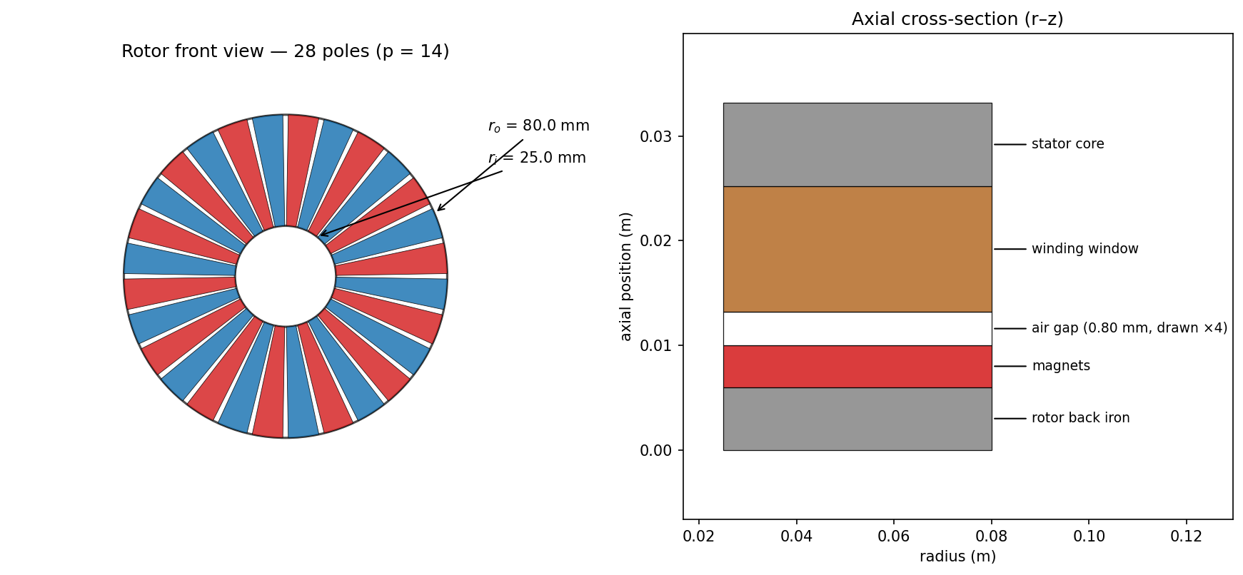
from axfluxmdo.viz import plot_geometry

motor = AxialFluxMotor(
    outer_radius=0.08,      # m
    inner_radius=0.025,     # m
    air_gap=0.0008,         # m
    pole_pairs=14,
    phases=3,
    turns_per_phase=24,
    fill_factor=0.45,
    magnet_thickness=0.004,        # m
    back_iron_thickness=0.006,     # m
)

op = OperatingPoint(speed_rpm=500, current_rms=25, dc_bus_voltage=48)

result = AnalyticalModel().evaluate(motor, op)
print(result)
plot_geometry(motor, show=True)

AnalyticalResult
  torque:            8.629 N·m
  torque density:    2.364 N·m/kg
  back-EMF (rms):    6.02 V/phase
  elec frequency:    116.7 Hz
  air-gap B:         1.016 T
  current density:   4.04 A/mm²
  copper loss:       20.0 W
  core loss:         0.91 W
  efficiency:        0.9557
  winding temp:      49.6 °C
  mass:              3.651 kg
  constraints:
    winding_temp_c: 49.57 <= 140 [OK, margin +64.6%]
    electrical_frequency_hz: 116.7 <= 1000 [OK, margin +88.3%]
    current_density_a_mm2: 4.042 <= 10 [OK, margin +59.6%]
    line_voltage_v: 10.9 <= 33.94 [OK, margin +67.9%]
    core_flux_density_t: 0.6696 <= 1.6 [OK, margin +58.2%]
    magnet_temp_c: 65 <= 80 [OK, margin +18.8%]

Key ideas visible already:

• The motor is a frozen dataclass. Variants are made with dataclasses.replace(motor, air_gap=0.001), the same mechanism sweeps and optimizers use, so nothing is ever mutated.
• Every result carries its constraint margins. result.feasible is the single boolean the optimizers honor; each named constraint reports a normalized margin.
• Results are flat dictionaries too. result.to_dict() keys (torque_nm, efficiency, winding_temp_c, ...) are a stable interface with short aliases (torque_density → torque_density_nm_kg) used throughout the optimization grammar.

Sweep something

from axfluxmdo.sweeps import sweep_parameter, sweep_pole_pairs

sweep = sweep_pole_pairs(motor, op, pole_pairs=range(4, 21, 2))
sweep.plot(show=True)

# dotted paths reach nested fields, e.g. manufacturing tolerances:
runout = sweep_parameter(motor, op, "tolerances.runout_m", [0, 1e-4, 2e-4, 3e-4])

Optimize

from axfluxmdo.optimize import optimize_pareto       # pip install "axfluxmdo[opt]"

study = optimize_pareto(
    motor, op,
    variables={
        "outer_radius": (0.05, 0.12),
        "pole_pairs": [8, 10, 12, 14, 16, 18, 20],
        "air_gap": (0.0005, 0.0015),
        "fill_factor": (0.30, 0.60),
    },
    objectives=["maximize_torque_density", "maximize_efficiency", "minimize_mass"],
    constraints=["winding_temp_c < 140", "electrical_frequency_hz < 1000"],
)
print(study.summary())

Tuples are continuous bounds, lists are discrete choices, objectives and constraints are strings over the result keys. Every returned design is feasible. See the optimization guide for the full grammar and Bayesian optimization for expensive objectives.

Where next

• The User Guide derives the physics each layer implements, with the equations and their code locations.
• The Examples are executed notebooks; every figure on this site regenerates from them.
• Limitations states what the fast models leave out, with FEA-measured error bars.